Laplacian matrix

In the mathematical field of graph theory the Laplacian matrix, sometimes called admittance matrix or Kirchhoff matrix, is a matrix representation of a graph. Together with Kirchhoff's theorem it can be used to calculate the number of spanning trees for a given graph. The Laplacian matrix can be used to find many other properties of the graph, see spectral graph theory. Cheeger's inequality from Riemannian Geometry has a discrete analogue involving the Laplacian Matrix, this is perhaps the most important theorem in Spectral Graph theory and one of the most useful facts in algorithmic applications. It approximates the sparsest cut of a graph through the second eigenvalue of its Laplacian.

1 Definition
2 Example
3 Properties
4 Deformed Laplacian
5 As a matrix representation of the negative discrete Laplace operator
6 As an approximation to the negative continuous Laplacian
7 See also
8 References

Definition

Given a simple graph G with n vertices, its Laplacian matrix 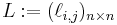$L:=(\ell_{i,j})_{n \times n}$ is defined as:^[1]

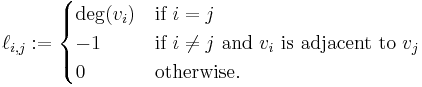
$\ell_{i,j}:= \begin{cases} \deg(v_i) & \mbox{if}\ i = j \\ -1 & \mbox{if}\ i \neq j\ \mbox{and}\ v_i \mbox{ is adjacent to } v_j \\ 0 & \mbox{otherwise}. \end{cases}$

That is, it is the difference of the degree matrix and the adjacency matrix of the graph. In the case of directed graphs, either the indegree or outdegree might be used, depending on the application.

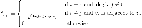
The normalized Laplacian matrix is defined as:^[1]

$\ell_{i,j}:= \begin{cases} 1 & \mbox{if}\ i = j\ \mbox{and}\ \deg(v_i) \neq 0\\ -\frac{1}{\sqrt{\deg(v_i)\deg(v_j)}} & \mbox{if}\ i \neq j\ \mbox{and}\ v_i \mbox{ is adjacent to } v_j \\ 0 & \mbox{otherwise}. \end{cases}$

Example

Here is a simple example of a labeled graph and its Laplacian matrix.

Labeled graph	Laplacian matrix
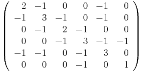	$\left(\begin{array}{rrrrrr} 2 & -1 & 0 & 0 & -1 & 0\\ -1 & 3 & -1 & 0 & -1 & 0\\ 0 & -1 & 2 & -1 & 0 & 0\\ 0 & 0 & -1 & 3 & -1 & -1\\ -1 & -1 & 0 & -1 & 3 & 0\\ 0 & 0 & 0 & -1 & 0 & 1\\ \end{array}\right)$

Properties

For a graph G and its Laplacian matrix L with eigenvalues 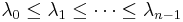$\lambda_0 \le \lambda_1 \le \cdots \le \lambda_{n-1}$ :

L is always positive-semidefinite ( $\forall i, \lambda_i \ge 0;\quad \lambda_0 = 0$ ).
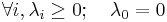The number of times 0 appears as an eigenvalue in the Laplacian is the number of connected components in the graph.
$\lambda_0$ is always 0 because every Laplacian matrix has an eigenvector of $[1,1,\dots,1]$ that, for each row, adds the corresponding node's degree to a "-1" for each neighbor, thereby producing zero by definition.
The smallest non-zero eigenvalue of L is called the spectral gap.
The second smallest eigenvalue of M is algebraic connectivity (or Fiedler value) of G.

If we define a signed edge adjacency matrix M with element M_ev for edge e (connecting vertex i and j, with i < j) and vertex v given by

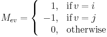
$M_{ev} = \left\{ \begin{array}{rl}1, & \text{if}\,v=i\\-1, & \text{if}\,v=j\\0, & \text{otherwise}\end{array}\right.$

then the Laplacian matrix L satisifies

$L = M^\text{T} M\,,$

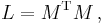
where $M^\text{T}$ is the matrix transpose of M.

Deformed Laplacian

The deformed Laplacian is commonly defined as

$\Delta(s)=I-sA%2Bs^2(D-I)$

where I is the unit matrix, A is the adjacency matrix, and D is the degree matrix, and s is a (complex-valued) number. Note that normal Laplacian is just $\Delta(1)$ .

As a matrix representation of the negative discrete Laplace operator

The Laplacian matrix can be interpreted as a matrix representation of a particular case of the negative discrete Laplace operator. Such an interpretation allows one, e.g., to generalise the Laplacian matrix to the case of graphs with an infinite number of vertices and edges, leading to a Laplacian matrix of an infinite size.

As an approximation to the negative continuous Laplacian

The graph Laplacian matrix can be further viewed as a matrix form of an approximation to the negative Laplacian operator obtained by the fdm. In this interpretation, every graph vertex is treated as a grid point, the local connectivity of the vertex determines the finite difference approximation stencil at this grid point, the grid size is always one for every edge, and there are no constraints in any grid points, which corresponds the case of the homogeneous Neumann boundary condition, i.e., free boundary.

References

^ ^a ^b Weisstein, Eric W., "Laplacian Matrix" from MathWorld.